Level 1 Report
2 / 11 / 2024
Basics
DataSet
1.Data set is used as a general term and can be of various formats - CSV file, databases, JSON, etc.)
2.Data sets is used in various contexts (ML, Data visualisation, statistics)
3.they need not always have tabular structure
DataFrame
1.Data structure Provided by Pandas Library
2.It represents data in a 2-dimensional, labeled data structure.
3.It comes with built-in functionalities for data manipulation, including filtering, grouping, aggregating, and more.
Outliers - Outliers are data points that differ significantly from the rest of the data in a dataset.
bias- when a machine learning model can represent the “true nature/ relationship" of the data.
high bias —> ML model does not fit the training data set (bad)
low bias —> ML model fits the training set (good)
variance- difference in fitting of training and testing data
high variance - large difference (bad)
low variance - lesser difference (good)
Ideally, our ML model has low bias and low variance.
Overfit - Overfitting occurs when a model learns the training data too well, including its noise and outliers. As a result, it performs excellently on the training data but poorly on test data.
Underfit - Underfitting occurs when a model is too simple to capture the underlying patterns in the data. It does not perform well on both training and test data.
The goal in machine learning is to find the right balance between overfitting and underfitting a.k.a bias-variance tradeoff.
Features: These are the independent variables or attributes (sometimes called columns or fields) used to make predictions. They represent the input data.
Instances: These refer to the rows, observations, data points, or cases in a dataset. Each instance represents a single observation with values for each feature.
Target: This is the dependent variable or response that you are trying to predict (also known as the predictant). It represents the output of the model based on the input features.
Supervised learning
When we explicitly tell a program what we expect the output to be, and let it learn the rules that produce expected outputs from given inputs, we are performing supervised learning.
- data is labeled and the program learns to predict the output from the input data
- pair of input object is a vector while the output value is a supervisory signal
- techniques include:
1. linear regression
2. logistic regression
3. multi- class classification
4. decision trees
5. SVM
regression is supervised learning in which the response is ordered and continuous, it finds correlation b/w independent and dependent variable , the variables are continuous
algorithms - simple linear regression , multiple linear regression , polynomial regression , support vector regression , decision tree regression and random forest regression
classification
-
category is the output
-
binary classifier (two outcomes)
-
multi - class classifier (multiple outcomes)
-
prediction of discrete values algorithms
-
linear models - logistic regression and support vector machines
-
non linear models - knn kernel SVM, naive bayes , decision tree classification , random forest classification eg: image classification(and captcha!)
Unsupervised learning- In unsupervised learning, we don’t tell the program anything about what we expect the output to be. The program itself analyzes the data it encounters and tries to pick out patterns and group the data in meaningful ways.
- data is unlabeled and the program learns to recognize the inherent structure in the input data
eg: clustering to create segments in a business’s user population. In this case, an unsupervised learning algorithm would probably create groups (or clusters) based on parameters that a human may not even consider.
Task 1 - linear and logistic regression
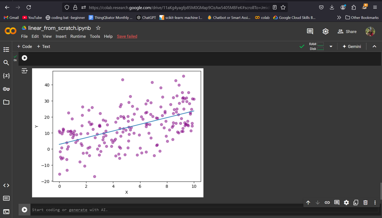
Linear Regression
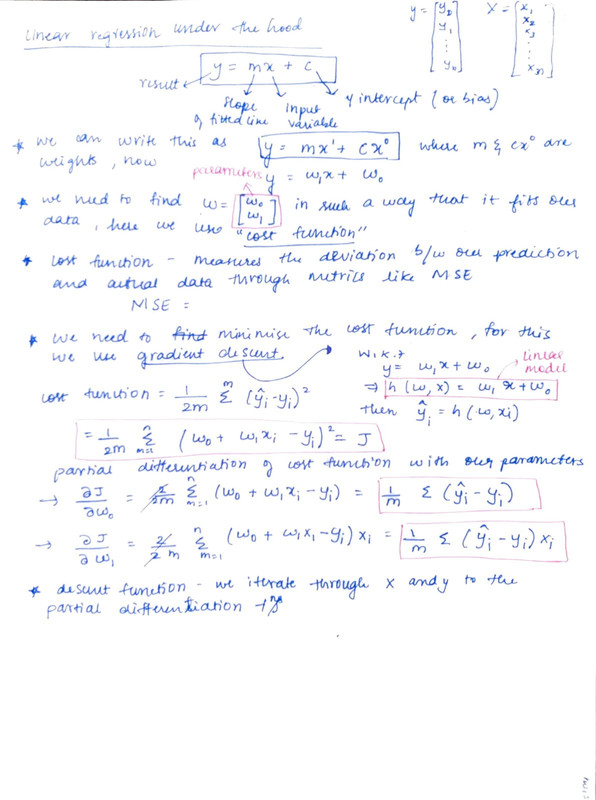
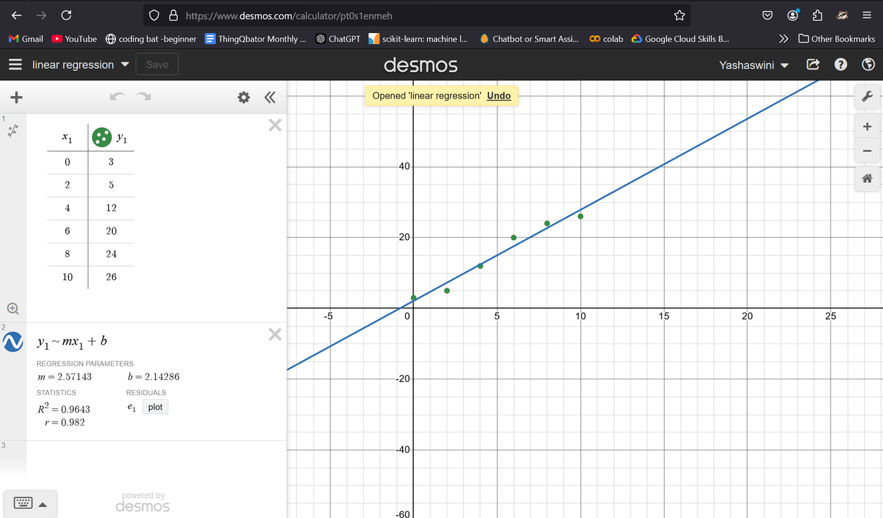
The goal of a linear regression model is to find the slope and intercept pair that minimizes loss on average across all of the data.
A line is determined by its slope and its intercept. In other words, for each point y on a line we can say:
y=mx+b
where m is the slope, and b is the intercept. y is a given point on the y-axis, and it corresponds to a given x on the x-axis.
(The slope is a measure of how steep the line is, while the intercept is a measure of where the line hits the y-axis.)
When we perform Linear Regression, the goal is to get the “best” m and b for our data. We will determine what “best” means in the following ways:
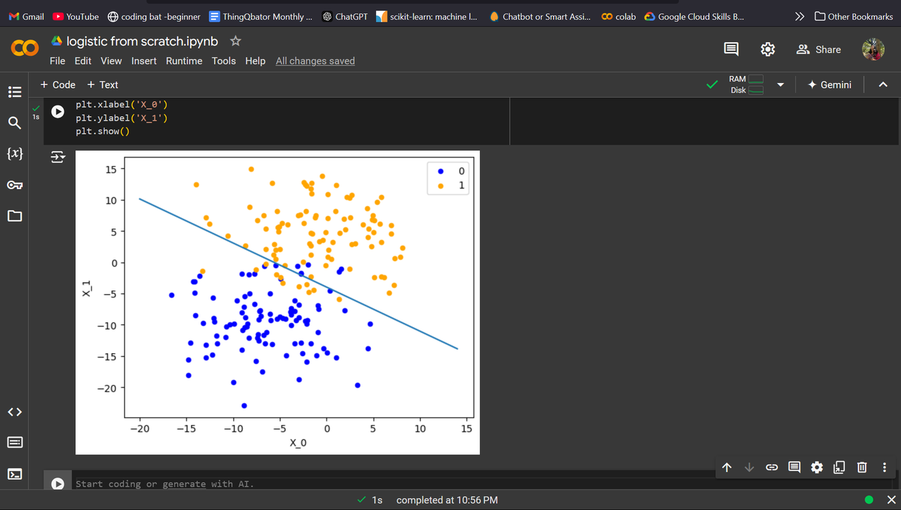
Logistic Regression
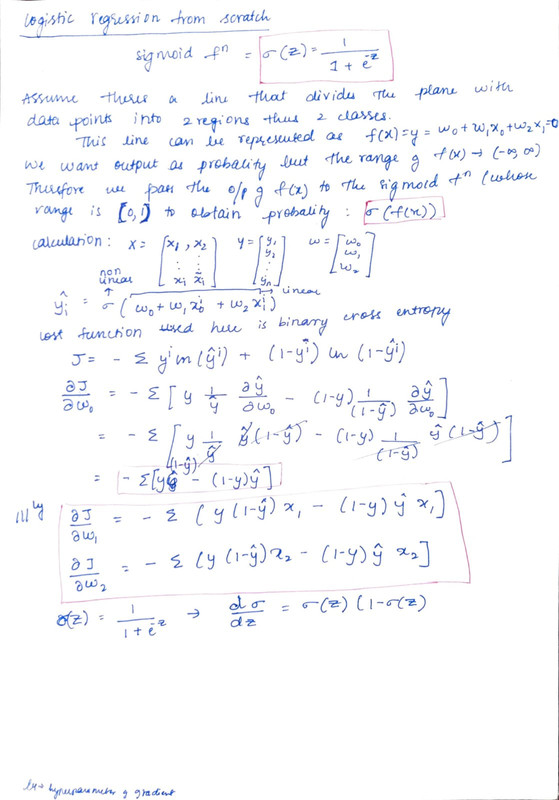
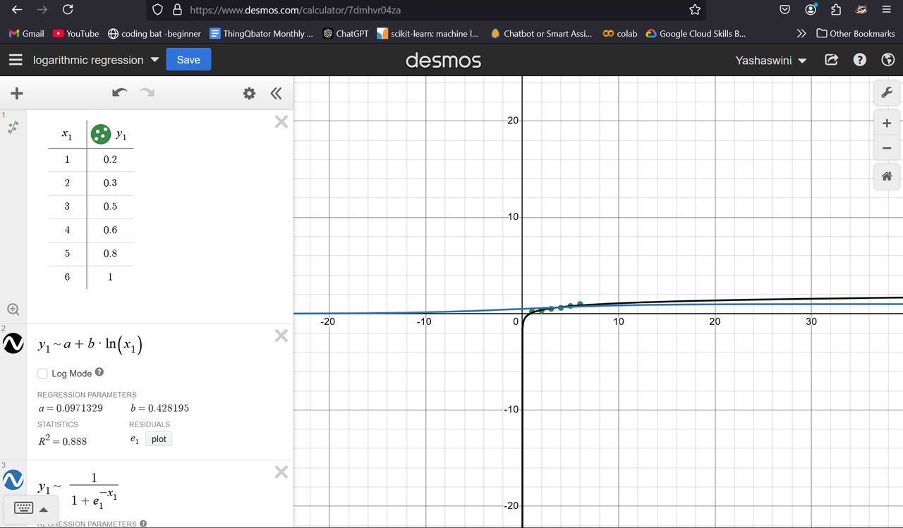
Logistic regression is a supervised machine learning algorithm that predicts the probability of a datapoint belonging to a specific category, or class in the range 0 to 1. These probabilities can then be used to classify data to the more probable group. Logistic Regression models use the sigmoid function to link the log-odds of a data point to the range [0,1], providing a probability for the classification decision. The sigmoid function is widely used in machine learning classification problems because its output can be interpreted as a probability and its derivative is easy to calculate.
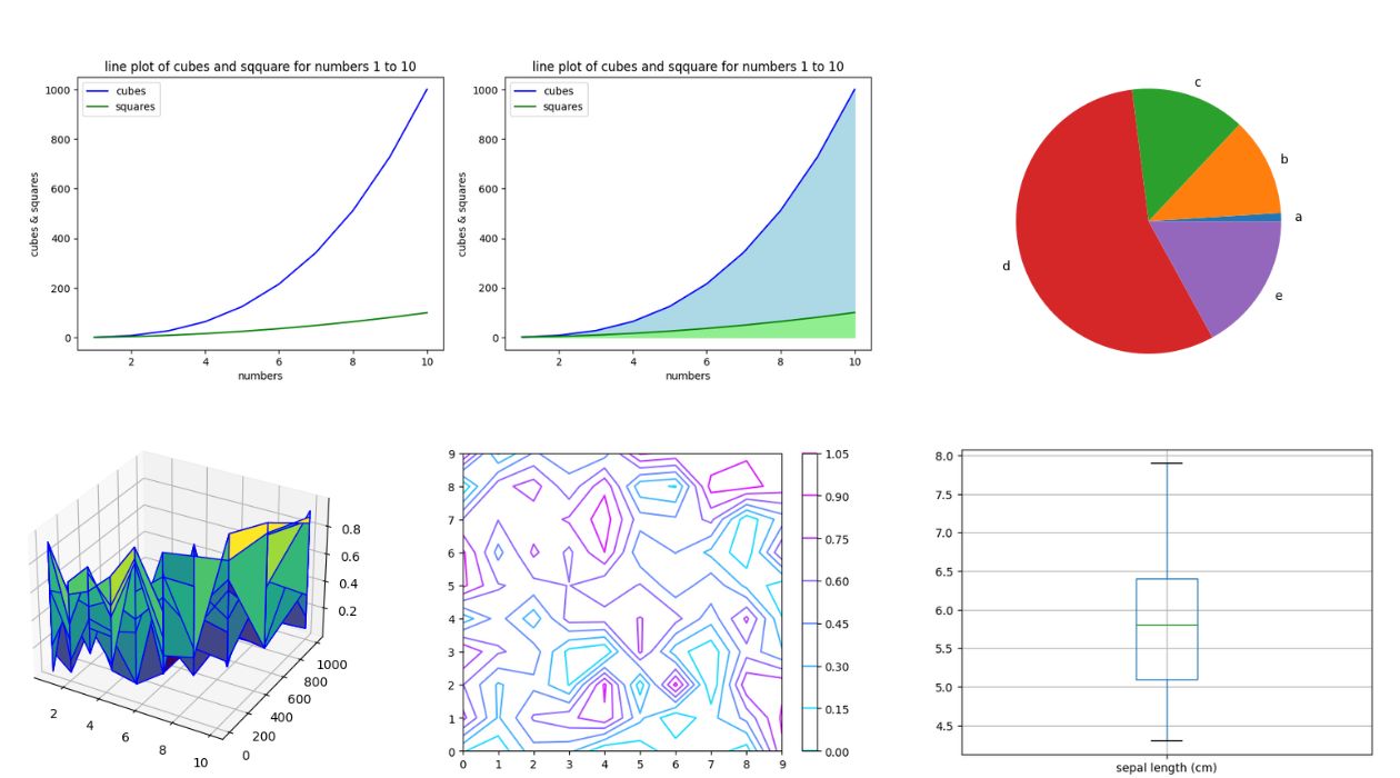
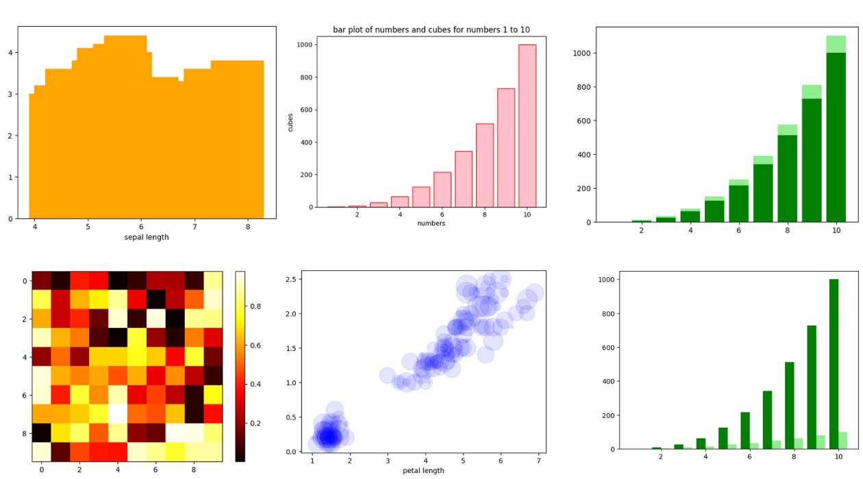
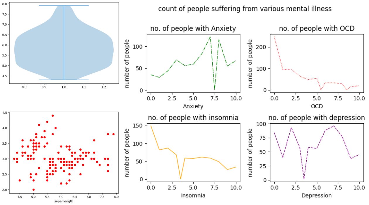
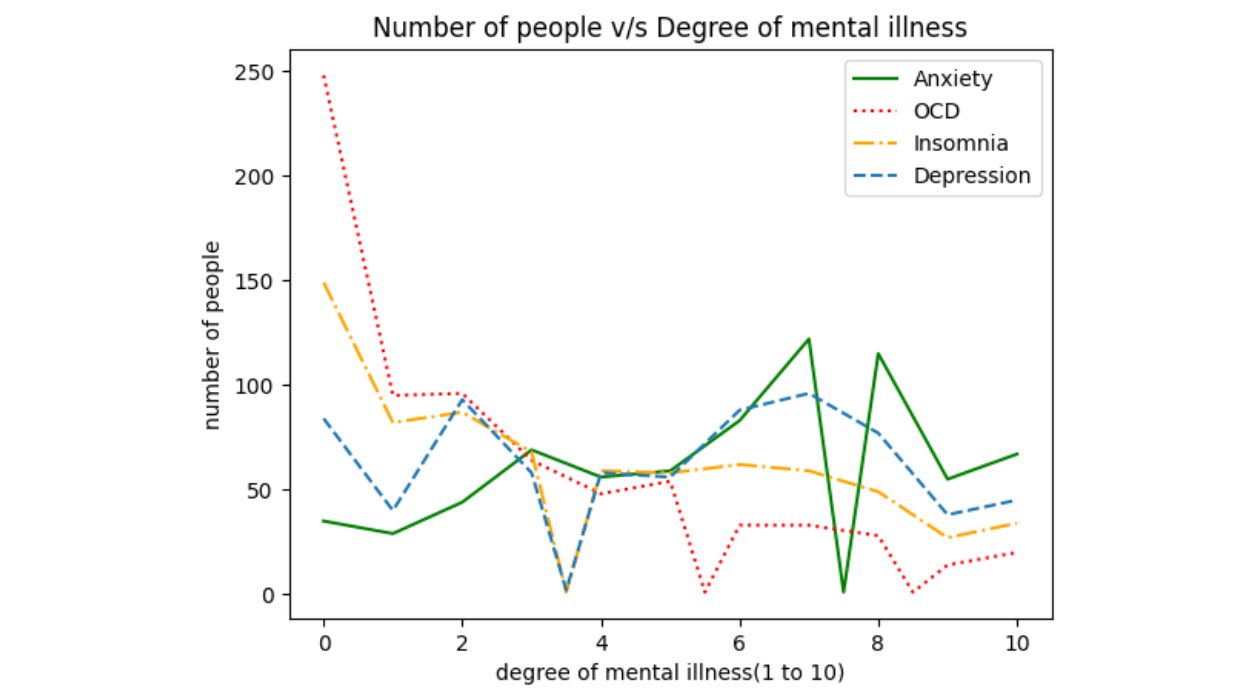
Matplotlib and Data Visualisation
Task 3 - NumPy
NumPy is a widely used Python library. It is used as it supports large, multidimensional arrays and also provides mathematical functions/operations such as linear algebra and statistical functions
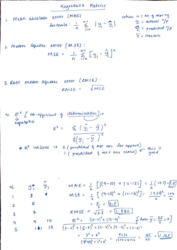
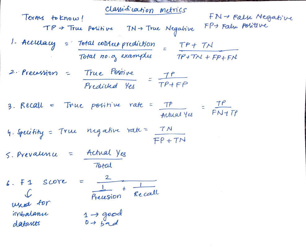
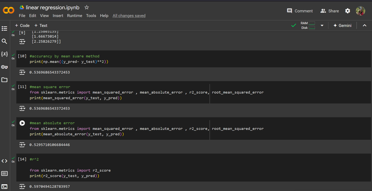
Task 4 - Metrics and Performance
Metrics plays a crucial part in any measurement process, not only does it gives the numerical value of a measurement, it also gives what that numerical value means.
for example, Celsius scale gives the temperature comparative to water's temperature while Fahrenheit scale gives the temperature comparative to human body (historically referenced).
Task 5 - Linear and Logistic Regression from scratch
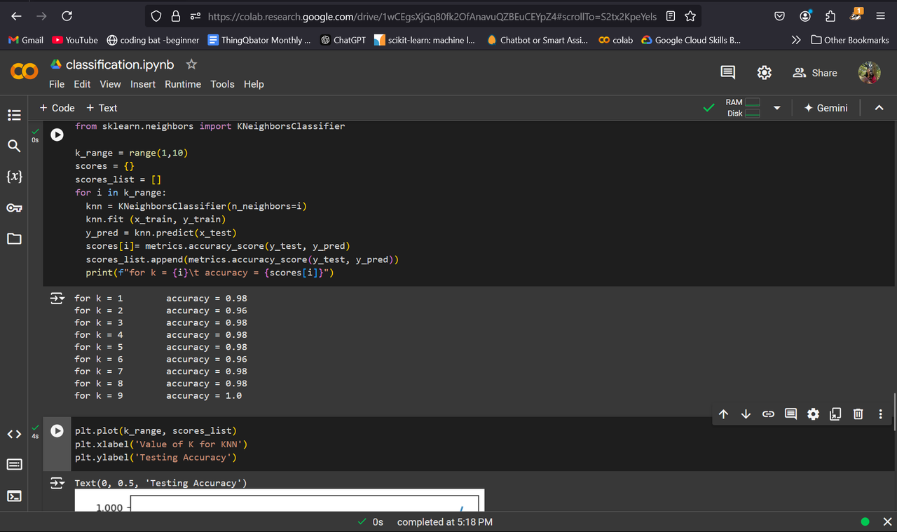
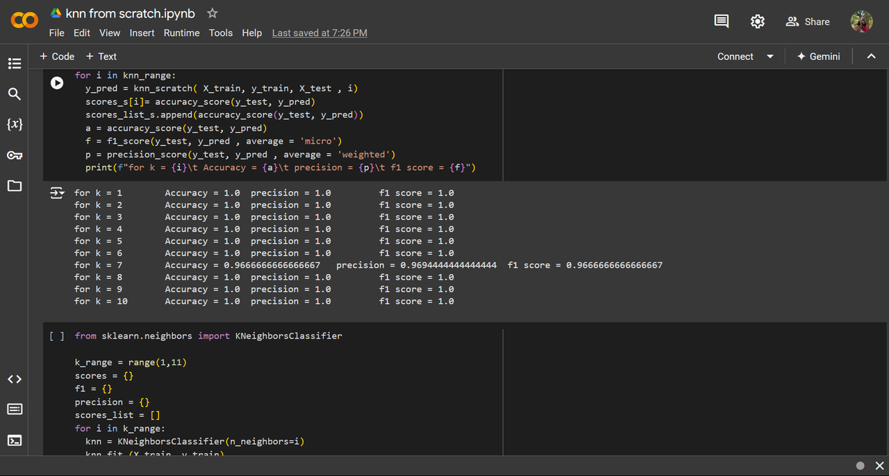
Task 6 - K Nearest Neighbor Algorithm
let's imagine a Srilankan who has a basic idea of Indian region and food, he/she thinks a north Indian person eats roti and a south Indian person eats masala dose, he/she makes an assumption on the food a person eats based on their geographical location. We now can easily predict that a punjabi eats roti and a kannadiga eats masala dose, but let's assume a person who lives in the middle of India (madya pradesh for namesake), equidistant from the region of roti and masala dose enthusiasts!
we can predict based on the madhya pradesh's neighbors' food habits, as a catch the sri lankan doesn't know it's neighbors and he starts to learn one by one in the decreasing order of nearness, this consideration of number of neighbors is denoted by the variable k and it takes the value of closest neighbor
the distance is measured by one of 2 popular methods -
- euclidean distance : D = sqrt((x_2 - x_1)^2 - (y_1-y_2)^2)
- Manhattan distance : D=∣x2−x1∣+∣y2−y1∣
Things to keep in mind while using KNN: - K value should not be a multiple of no. of classes to avoid tie between classes
- When using distance metrics, the scaling of the axes (features) is crucial. If features are on different scales (e.g., age in years and income in thousands), distances may be dominated by features with larger ranges. Use normalization technique or standardization.
- as the dataset increases, the complexities increases. make this complete
Task 7 - An elementary step towards understanding Neural Networks
Task 8 - Mathematics behind machine Learning
what is models in aiml?
modeling refers to the process of creating a mathematical representation of a data set.
to model a data set, we need to understand our problem statement clearly ( like if we want it to classify or predict) then selecting appropriate features (input variables). we then have to find an algorithm based on our problem statement and data.
We have to train the algorithm on our data and use metrics to evaluate it’s performance. we can then tune the model to make better prediction. this whole process is called modelling and it is the core part of machine learning processes.
curve fitting
Curve fitting is a statistical technique used to create a mathematical model that best represents the relationship between variables in a dataset. It is used to identify and describe relationship b/w features/independent variables and target/ dependent variables, then we could use this relationship to predict and analyse the data.
 function approximators
Function approximators are mathematical models or algorithms used to estimate or approximate a target function based on input data. It enables us to generalise from a finite training data to predict unseen data. Thus they form a backbone of many ml algorithms that includes regression, classification, and reinforcement learning.
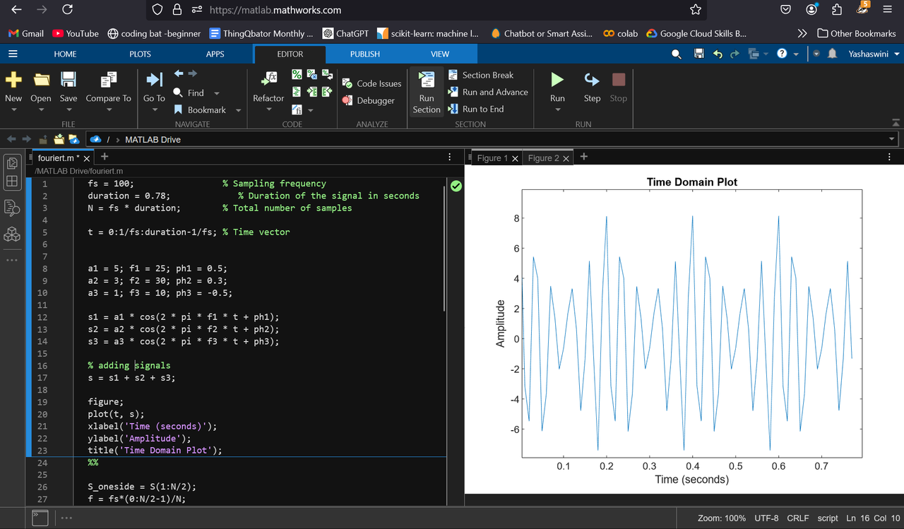
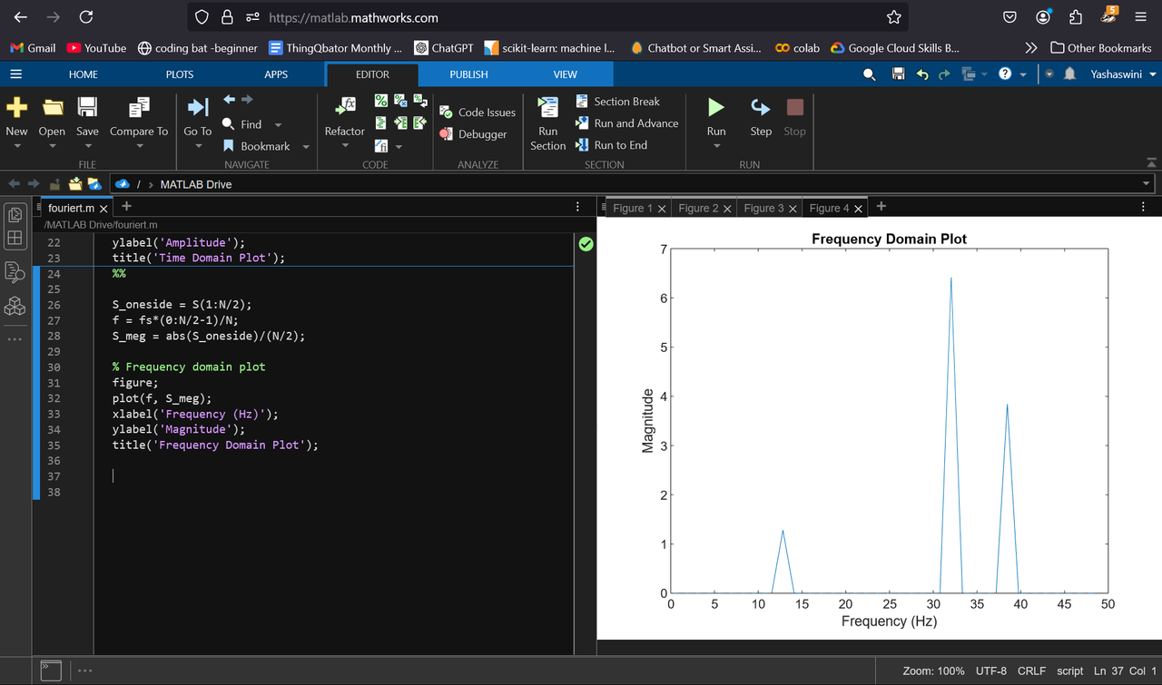
fourier transform in aiml
The Fourier transform is an important tool in AIML as it could be used for analysis and processing of signals and images (enabling speech recognition and image compression). It is very useful in trend detection in time- series data.
Task 9 - Data Visualization using Plotly
Task 10 - An introduction to Decision Trees
decision tree works on the principle of determined based on true or false
- classification tree - decision tree classifies into categories
- regression tree - decision tree classifies into numeric values
- Root Node , internal nodes/Branches , leaf nodes
- deciding root node is important and we can determine it by comparing different types of data and select the one which has “purity” in them
- purity/ Impurity can be determined by several methods such as Gini Impurity, Entropy and Information Gain
- Gini Impurity for leaf = 1 - (probablity of “true/Yes”)^2 - (the probablity of “false/ no”)^2
- Total Gini impurity = weighted average of gini impurity of leaves
- weight = total observations in one leaf / total observations in both the leaf
- we choose the lowest impurity for root node
Task 11 - SVM
- the shortest distance between the threshold and the observation is called as margin
- Maximal margin classifier - when the margin is exactly between the edges of the cluster
- problems with maximal margin classifier is that it is sensitive to outliers and thus the margin will lie in a different place than intended to.(not good)
- Misclassification should be allowed to make maximum margin classifier insensitive (bias - variance tradeoff) thus we get a soft margin.
- cross validation is used to determine the soft margin that allows least number of misclassification.
- Soft margin classifier == support vector classification (here support vector are the observation on the edge and within the soft margin)
- hyperplane is a line that represents the margin that divides the data set
support vector machine start with data in relatively low dimensions and move the data to a higher dimension then find the support vector classifier to classify the data.We find the correct function to move the data to higher dimension by systematically using kernel functions.
I had a learning curve in this level but I found everything super interesting :)

