Level 2
17 / 9 / 2024
Task 1 - Linear and Logistic Regression
Linear Regression
Linear regression is a data analysis technique that predicts the value of unknown data by using another related and known data value.
To predict the price of a home, based on multiple different variables
Work
Logistic Regression
Logistic regression is a data analysis technique that uses mathematics to find the relationships between two data factors. It then uses this relationship to predict the value of one of those factors based on the other.
Train a model to distinguish between different species of the Iris flower based on speal length and width and petal length and width
Work
Task 2 - Matplotlib and Data Visualisation
Matplotlib
Matplotlib is a low level graph plotting library in python that serves as a visualization utility.
Explore the various basic characteristics to plots as given below, with python libraries:
- Set axes label
- Set axes limits
- Create a figure with multiple plots using subplot
- Add a legend to the plot
- Save your plot as png
Explore the given plot types:
- Line and Area Plot
- Scatter and Bubble Plot using Iris dataset
- Bar Plot • Simple • Grouped • Stacked
- Histogram • Pie Plot • Box Plot • Violin Plot • Marginal Plot • Contour Plot • Heatmap • 3D Plot
Work
Task 3 - Numpy
Numpy
NumPy is a Python library used for working with arrays. It also has functions for working in domain of linear algebra, fourier transform, and matrices.
In Python we have lists that serve the purpose of arrays, but they are slow to process. NumPy aims to provide an array object that is up to 50x faster than traditional Python lists.
Using Numpy Generate an array by repeating a small array across each dimension and Generate an array with element indexes such that the array elements appear in ascending order.
Work
Task 4 - Metrics and Performance Evaluation
Regression Metrics - used to evaluate performance of regression algorithms
Classification Metrics - used to evaluate performance of classification algorithms
Regression Metrics:
Regression models predict continuous numerical values, and scikit-learn provides various algorithms like Linear Regression, Decision Trees, Random Forests, and Support Vector Machines (SVM).
Evaluation of Regression Metrics:
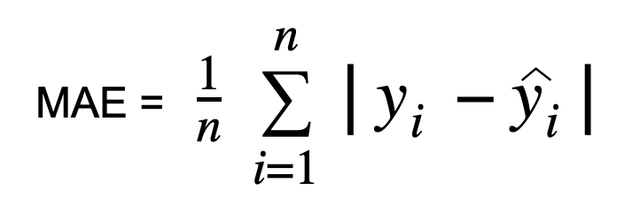
Mean Absolute Error (MAE): Measures average absolute differences between actual and predicted values.
 Mean Squared Error (MSE): Measures average squared differences between actual and predicted values.
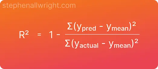
 R-squared (R²) Score: Indicates the percentage of variance in the dependent variable explained by independent variables.
 Root Mean Squared Error (RMSE): Measures the square root of the MSE.

Classification Metrics:
Classification metrics are used to evaluate the performance of classification models. These metrics provide insights into how well the model is performing in terms of correctly classifying instances into different classes.
Evaluation of Classification Metrics:
Accuracy: Measures the proportion of correctly predicted instances out of the total instances.
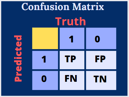
Confusion Matrix: A confusion matrix is a table that visualizes the performance of a classification model. It presents a summary of the predicted versus actual class labels. The rows represent the actual classes, while the columns represent the predicted classes. The confusion matrix consists of four metrics:
• True Positive (TP): The number of instances correctly predicted as positive.
• True Negative (TN): The number of instances correctly predicted as negative.
• False Positive (FP): The number of instances incorrectly predicted as positive (Type I error).
• False Negative (FN): The number of instances incorrectly predicted as negative (Type II error).
 Classification Report: It includes metrics such as precision, recall, F1-score, and support for each class. These metrics are calculated based on true positive (TP), false positive (FP), true negative (TN), and false negative (FN) predictions.
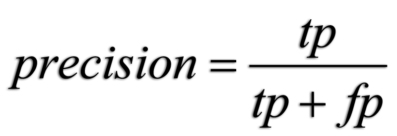
Precision: Precision measures the proportion of correctly predicted positive instances out of all instances predicted as positive. It is calculated as
 Recall (or Sensitivity): Recall measures the proportion of correctly predicted positive instances out of all actual positive instances. It is calculated as
 F1-score: The F1-score is the harmonic mean of precision and recall. It provides a balance between precision and recall. It is calculated as
 Support: Support is the number of actual occurrences of the class in the specified dataset.
Work
Task 6 - K- Nearest Neighbor Algorithm
Task
Understanding the algorithm Implement KNN from scratch Implement KNN using sci-kit’s neighbors.KNeighborsClassifier for multiple suitable datasets and compare results with sci-kit’s built in method for different datasets.
Procedure
1.Define KNN class: We define a class named KNN to implement the K-Nearest Neighbors algorithm. This class contains methods for fitting the model (fit()), calculating Euclidean distance (euclidean_distance()), and making predictions (predict() and _predict()).
2.Implement Euclidean Distance: The euclidean_distance() method calculates the Euclidean distance between two points using NumPy's vectorized operations.
3.Fit the Model: The fit() method takes the training data as input and stores it internally within the KNN object.
4.Predict Method: The predict() method predicts the labels for a given set of input samples. It iterates through each sample and calls the _predict() method to make individual predictions.
5.Predict Single Sample: The _predict() method predicts the label for a single sample by calculating distances to all training samples, selecting the k nearest neighbors, and returning the most common label among them.
6.Compare with scikit-learn's KNeighborsClassifier: We load three different datasets: Iris, Digits, and Wine. For each dataset, we split the data into training and testing sets using train_test_split().
7.Train and Evaluate Models: For each dataset, we train scikit-learn's KNeighborsClassifier and our custom KNN implementation on the training data and evaluate their performance on the testing data using accuracy.
8.Print Results: We print the accuracy of both models for each dataset, allowing us to compare their performance.
Work
https://colab.research.google.com/drive/1E-g6Kw4cnWY1DPHT7CeHhe5HfL2-ybpO?usp=sharing
Task 7: An elementary step towards understanding Neural Networks
• Write a blog about your understanding of Neural Networks and types like CNN, ANN, etc. Make sure to include any mathematical implication. You can add the function calls used to implement the algorithms. •Learn about Large Language Models at a basic level and make a blog post explaining how you would build GPT-4.
Blog link: https://hub.uvcemarvel.in/article/6d05f7d3-c2de-4886-906a-9b248b9fdc1c
Task 8: Mathematics behind machine learning
Task
☆ Curve-Fitting- Model a curve fitting for a simple function of your choice, on Desmos.
☆ Fourier Transforms- Fourier transforms are perhaps the most important function approximators used today. Model a fourier transform for a function of your choice on MATLAB.
Task 9: Data Visualization for Exploratory Data Analysis
Use Plotly for data visualization. This is an advanced visualization library, more dynamic than the generally used MatPlotlib or Seaborn.
https://colab.research.google.com/drive/1rE8GDc2eL5M_mI3QMFbwZYSnGcbFjoc3?usp=sharing
Task 10: An introduction to Decision Trees
Loading the Dataset: We start by importing the necessary modules from scikit-learn. We load the Iris dataset using load_iris() function from scikit-learn's datasets module. This dataset contains features (sepal length, sepal width, petal length, and petal width) of iris flowers and their corresponding labels (species). Splitting the Data: We split the dataset into training and testing sets using train_test_split() function from scikit-learn's model_selection module. The parameter test_size=0.2 specifies that 20% of the data will be used for testing, and the rest for training. The parameter stratify=y ensures that the splitting is done in a stratified fashion, meaning that the class distribution is preserved in both the training and testing sets. Initializing the Decision Tree Classifier: We initialize a DecisionTreeClassifier object from scikit-learn's tree module. We set random_state=42 to ensure reproducibility of results. Training the Classifier: We train the decision tree classifier on the training data using the fit() method, where X_train contains the features and y_train contains the corresponding labels. Making Predictions: We use the trained classifier to make predictions on the testing data using the predict() method. The predicted labels are stored in y_pred. Calculating Accuracy: We calculate the accuracy of the classifier by comparing the predicted labels (y_pred) with the true labels (y_test) using the accuracy_score() function from scikit-learn's metrics module. The accuracy score represents the proportion of correctly predicted labels in the testing set. Cross-Validation: We use cross-validation to evaluate the model's performance more reliably. This is done using the cross_val_score() function from scikit-learn's model_selection module. The parameter cv=5 specifies 5-fold cross-validation, where the dataset is split into 5 folds, and the model is trained and tested 5 times, each time using a different fold as the testing set. The mean of the cross-validation scores (cv_scores.mean()) provides an estimate of the model's generalization performance. Overall, this code demonstrates the process of training and evaluating a decision tree classifier on the Iris dataset, including data splitting, model training, prediction, accuracy calculation, and cross-validation for performance evaluation.
https://colab.research.google.com/drive/14h0hzS-WxJtD1ruohsJHTsA4JjFUv-t4?usp=sharing
Task 11: Exploration of a Real world application of Machine Learning
Algorithms trained by a student taking their first steps into Machine learning are vastly different from algorithms used for professional deployment. Find out what’s on the market, and why it’s on the market, i.e. take a real world project and document the use of Machine Learning algorithms and mathematical constructs used in it.This task can be done as a case study.
https://hub.uvcemarvel.in/article/b7d98f69-1787-4ec9-a84b-98cdaf9563dc
