
BLOG · 3/6/2025
NEURAL NETWORKS
A high level walkthrough of neural networks

Neural Network
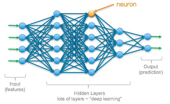
It is a computational model that uses several layers of interconnected neurons to make various types of predictions, recognize patterns, and perform tasks like speech recognition, translation, etc.
Neurons – A neuron is simply a function that holds a value between 0 and 1. This value is the activation of the neuron.
A typical neural network has three types of layers:
Input layer – It receives the raw data, and the activation in the neuron is dependent on the input.
Hidden layers – Every neuron is connected to every other neuron in the next layer. Their activations are calculated using the sigmoid function. Each layer is associated with recognizing some features of the input, which in turn stimulate bigger features in the next layer and so on until the output is predicted in the output layer. This activation is calculated by taking the sigmoid of the sum of the products of activations in the previous layer with the weights and the bias. The weights are what push the activation of the neuron, and the bias determines how easy or hard it is to activate the neuron.
Output layer – It is the final layer where the neuron with the maximum activation is the output.
Loss function
Obviously, it is unlikely that the correct output will be given in the first trial of the forward propagation, given that there are a huge number of inputs compared to a single output. So, we make nudges to the weights and biases to change the activations in the further layers and bring about values that almost perfectly give the right output. How wrong our prediction is can be computed using a loss function. We can use MSE or cross-entropy classification for this purpose.
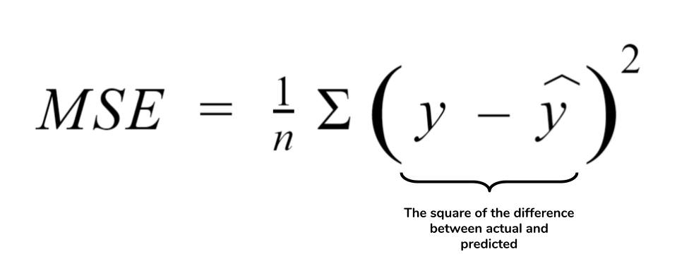
MSE ( Mean squared error)– It is the difference between the favorable output and the incorrect output, squared and then averaged.
To minimize this loss, we use backpropagation and achieve gradient descent (finding the local minimum of a cost function).
We know that taking the negative derivative of the cost function gives us the minimum of that function. This tells us how the weights and biases must be changed so that the cost function is minimized.
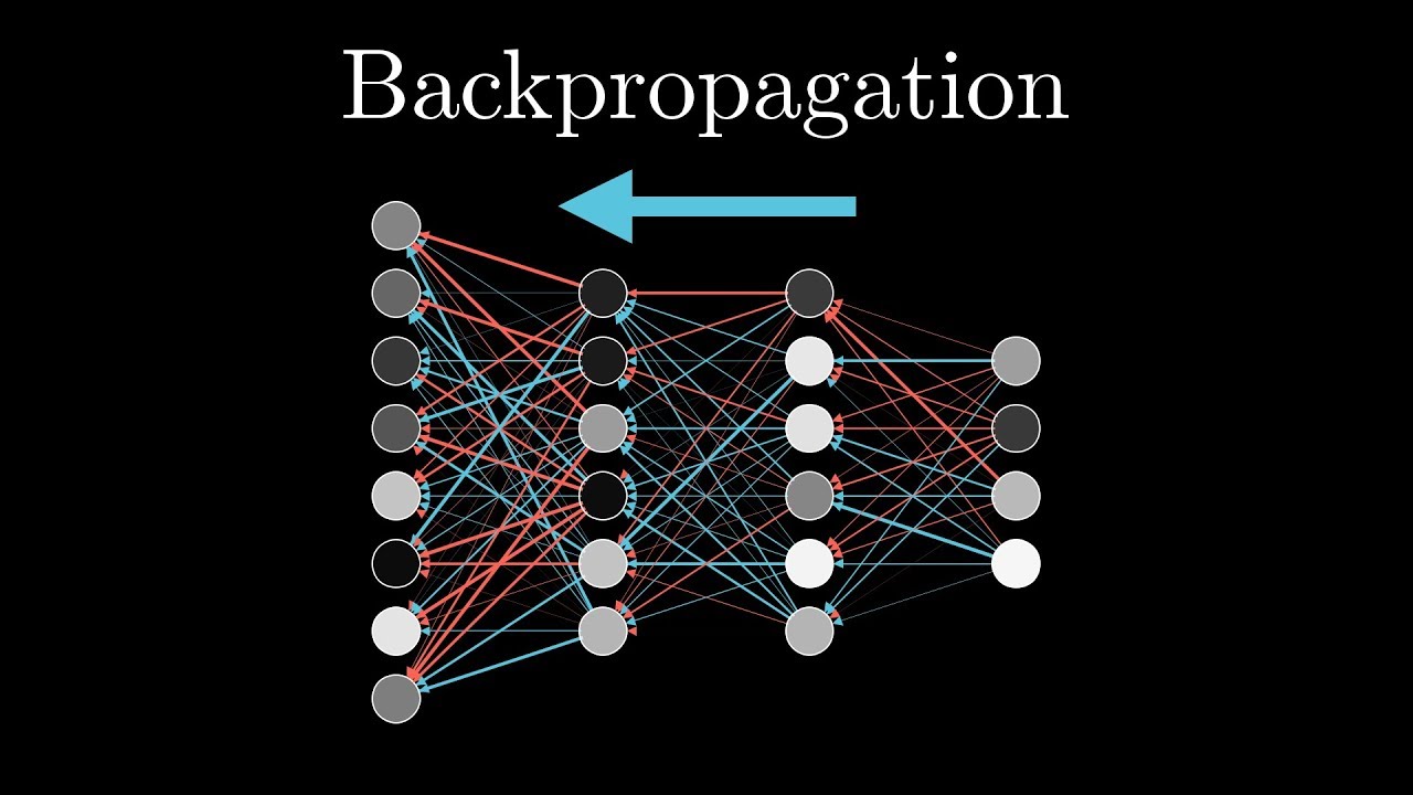
Backpropagation
For a given training data point, each neuron has an opinion on how the activations in the previous layer should be. The sum of these gives the idea of how much change is needed for each neuron in that previous layer. Now, each training data point gives such opinions. Averaging these gives the negative gradient of the cost function. For speeding up computation, we can make use of stochastic backpropagation.
Types:
FNN– Data flows in a single direction from input → hidden layers → output, without loops or feedback. It is simple and easy to implement for non-sequential data and is good for classification and regression purposes.
CNN – Mainly used for recognizing and processing visual data, object detection, and facial recognition. It uses convolutional layers with filters to scan the image and detect patterns, which are then passed through fully connected layers to make predictions. It also uses pooling layers to reduce the size of the data, which speeds up processing and makes the network more efficient.
from tensorflow.keras.layers import Conv2D, MaxPooling2D, Flatten

model = Sequential([
    Conv2D(32, (3,3), activation='relu', input_shape=(28,28,1)),
    MaxPooling2D(pool_size=(2,2)),
    Flatten(),
    Dense(64, activation='relu'),
    Dense(10, activation='softmax')
])
ANN – ANNs typically have an input layer, one or more hidden layers, and an output layer. As data flows through the network during training, the ANN adjusts its weights and biases to minimize the error between its predictions and the correct answers. Unlike CNNs, ANNs consist entirely of fully connected layers.
from tensorflow.keras.models import Sequential
from tensorflow.keras.layers import Dense

model = Sequential()
model.add(Dense(64, activation='relu', input_shape=(100,)))
model.add(Dense(32, activation='relu'))
model.add(Dense(10, activation='softmax'))
RNN– RNNs have the ability to remember previous inputs through an internal memory called a hidden state, which is updated at each step of the sequence. Based on the current input and this memory, the RNN makes a prediction or decision at each step. This step-by-step processing with memory is what allows RNNs to understand sequences and patterns over time.
from tensorflow.keras.layers import SimpleRNN

model = Sequential([
SimpleRNN(50, activation='tanh', input_shape=(100, 1)),
Dense(1)
])