An Introduction to Neural Networks

INTRODUCTION AND BASICS

Neural networks are a subset of machine learning, underneath which comes the concept of deep learning— Which I'm sure are terms we've all heard before at some point, but might've sounded too daunting to delve into the details of. Before getting into the intricacies of neural networks, let's first understand how this links to concepts that we're already relatively familiar with.

Machine learning is just that— Teaching a machine how to think and come to conclusions as a result of data retention and pattern recognition. To put it simply, the process of "teaching" a machine can be gone about in multiple ways. One of these ways is by developing a Neural Network; A concept inspired by the networks in the human brain.

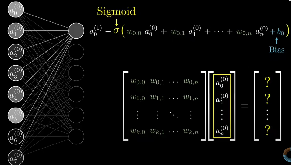
Essentially, this method of ML involves a bunch of layers of information stored in units, called neurons. There are three main layers— The input layer, hidden layers (yes, plural) and an output layer. Each of these layers contain neurons carrying some value, and every neuron is connected to neurons of the succeeding layer. Each connection carries some 'weight', which is a factor which the value of the neuron is multiplied by. The weighted sum of every neuron in the focus layer is taken, and another value known as 'bias' is added to this weighted sum. As a whole, this is called the activation function. This process occurs layer-by-layer, until the output layer is reached and some value is obtained. This value is essentially a probability. The neuron in the output layer with the highest probability is taken as the output for this particular round, and compared with the true output.



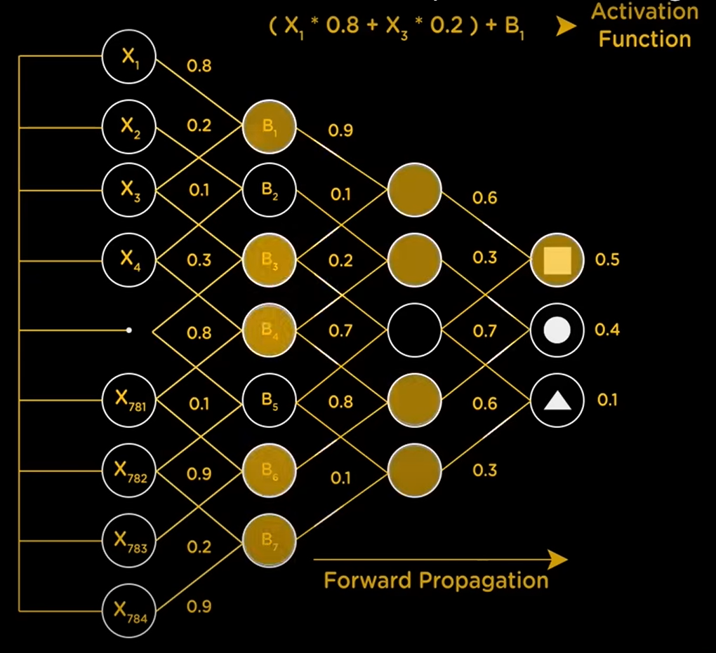
If the output doesn't match the true output, then the weights and biases are adjusted dynamically after every round until the actual output is obtained. This is the training process. Once the model has been trained, it is ready to receive test data, using which it'll make predictions. We can deepen our understanding of this concept using an example.

Assume that we've got an image, 15x15px. This amounts to 225 pixels in the entire image. Now let's suppose that we've multiple images of some basic shapes, and we'd like the model to determine which shape is in the image.

If the shapes under consideration are a square, circle and triangle, we'll claim our output layer to consist of them. The layer right before the output layer (nth hidden layer) would contain the basic features that make up each of these shapes— a horizontal line, a vertical line, a curve, and diagonal lines. If the weighted sum of the horizontal line + vertical line features are the highest, it implies that the shape in question is a square. Similarly, if the weighted sum of the horizontal line + diagonal lines features are the highest, the shape in question would be a triangle.



Now, the layer before the nth hidden layer [(n-1)th hidden layer] would have the features of the nth hidden layer's components, i.e., it would have the features (horizontal line, vertical line, etc) broken down into smaller segments/smaller features. So, it would contain a fraction of the pixels that make up each of the lines in the nth hidden layer. To illustrate this visually, we can say that a horizontal line may be divided into halves. Let's say that this horizontal line is the base of a square. This implies that the bottom couple of pixels would be occupied by the horizontal line. We have now divided this horizontal line into two halves, and similarly, every other feature (curve, diagonal line, etc.) into halves as well. These halves make up the (n-1)th hidden layer. When we take the weighted sum of these neurons, if we get the maximum values as those of the two haves of the horizonal line, we'll know that that's the feature to be selected in the nth hidden layer.

This process is repeated for every single layer that exists in the network, and it's all dynamically amended. Ergo, we can obtain very accurate results as the number of iterations increase.

Now, as for how exactly this works on the numerical level, now that we've understood the basic concept— Let's say that the image containing the shape has a black background, and the shape is hand-drawn in white. Every pixel will have an assigned value between 0 and 1 (to align with the whole 'probability' concept, and for simplicity's sake), where 0 stands for a fully black pixel, 1 stands for a fully white pixel, and any decimal values in between are grey areas. The probability values of fully white/close to fully white pixels will obviously be greater than that of grey pixels. Using this, we can conclude that grey pixels are like the borders to our features (such as the lines, as discussed earlier). The darker the grey of the pixel visually, the lower its value gets, and its probability of being considered a border region increases. This process is called edge detection. The values of the neurons are called activations. It's worth noting that weights may be a positive or a negative value. The weights associated with white pixels/neurons will be on the positive side, and the weights of all the surrounding pixels or the border, will be more negative.

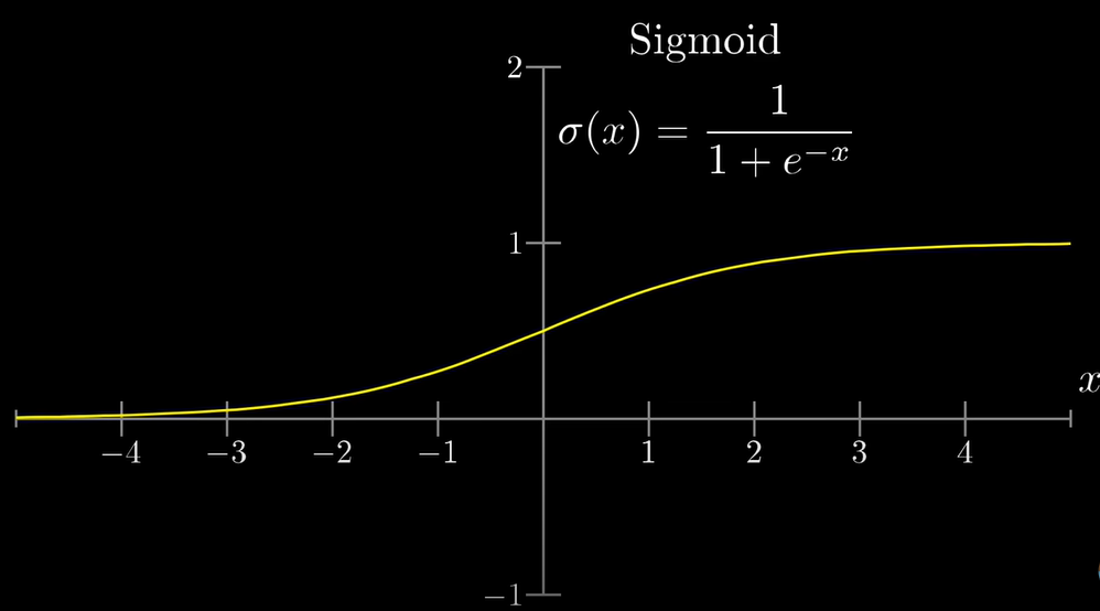
Let's look at some more math here. We now have our weighted sum. But what we don't have, is the guarantee that this sum will be a number between 0 and 1— But we need a number between 0 and 1, since we're just taking the whole concept as a function of probability (i.e., we're essentially finding the probability of the given shape being one of our three output shapes. Also, the activation of every neuron is always a value between 0 and 1). In order to make sure that the weighted sum lies within this range, we somehow need to 'smoosh' the weighted sum function into the range [0, 1]. To do this, we use the sigmoid function (which we used in logistic regression in an older task!). This function throws outputs as follows: Very negative inputs end up being close to 0, and very positive inputs are closer to 1, and that's that.



I'd also like to recall that we included a 'bias' when we first took our weighted sum. Let's look at why we need this parameter in our already annoying-looking equation. We can establish from all the yapping above, that the activation of a neuron multiplied by some weight, will basically give us a measure of how positive the activation of a neuron in the next layer is, i.e., it'll tell us how high the probability of aq certain feature existing in the next layer is. For example, if the value of the neuron containing the upper half of a diagonal line is high, then in the next layer (which contains full lines), we can conclude that the value of the neuron containing a full diagonal line is high. This is convenient for simple networks. However, with networks containing identical features and more details, we might want neuron activations which have slightly higher values. For our three-shape example, we may be happy if our weighted sum is some value above 0. But in other instances where most values of the sum are above 0, our threshold might be that we need a sum above 10. To achieve this, we add a bias to the vanilla weighted sum. So this ensures that a certain neuron in the next layer only gains activation when (weighted sum + bias > 10).

To sum this part up, the weight tells us how positive a neuron's value is, and the bias gives us a meaningful threshold to actually activate a neuron in the next layer. It is important to note that these weighted sum and bias shenanigans are performed before plugging the entire value into the sigmoid function, which, incidentally, will produce a logistic curve when plotted.

We'll now discuss a concept I should've talked about before but genuinely forgot to add: How many neurons and weights and biases exist in each layer, or between one layer to the next?

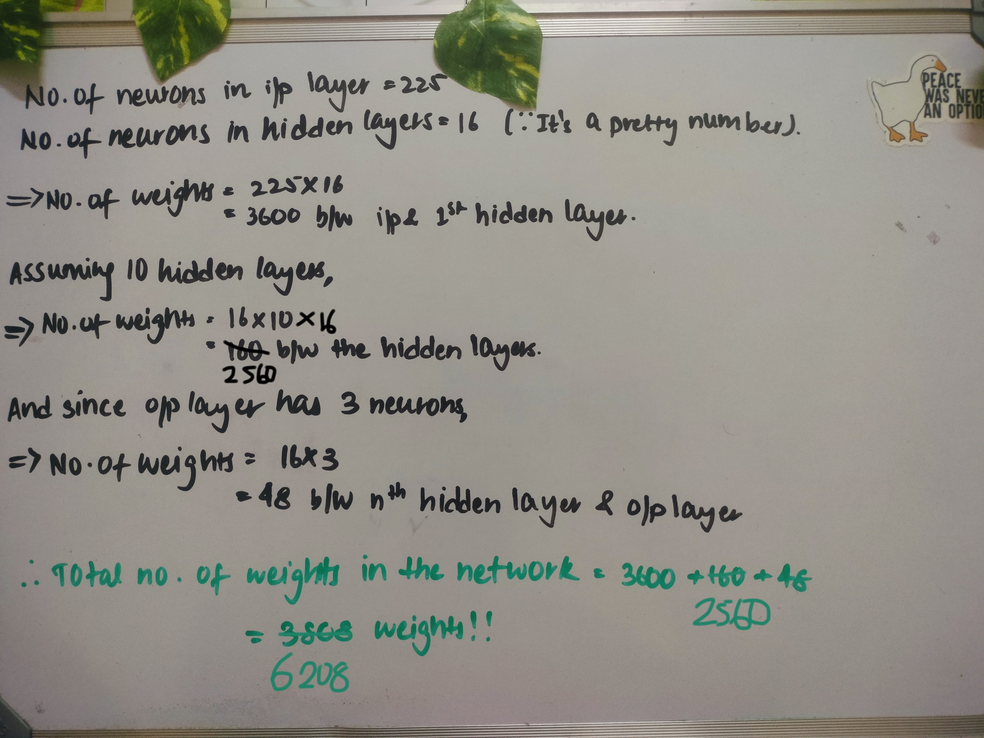
• Input layer: We discussed earlier that the image is 15x15px, which equals 225 pixels overall. => The input layer will have 225 neurons.
• Output Layer: We have three possible outputs with the example we've taken. => The output layer will have 3 pixels.
• Hidden Layers: The choice of the number of hidden layers is a balancing act, of sorts. We can start by selecting some value between the number of input and output layers, and adjust according to how the model performs. If we notice any overfitting, we can reduce the number. If the model isn't able to learn the data at all, we can increase the number. => Good luck figuring out the number of neurons in the hidden layers.
  
• Weights: Every neuron is connected to every other neuron in the next layer. So one neuron in the 1st hidden layer will be connected to all 225 neurons in the input layer. Thus, this one neuron in the 1st hidden layer will have 225 weights that are included to give the weighted result required, which is its activation.
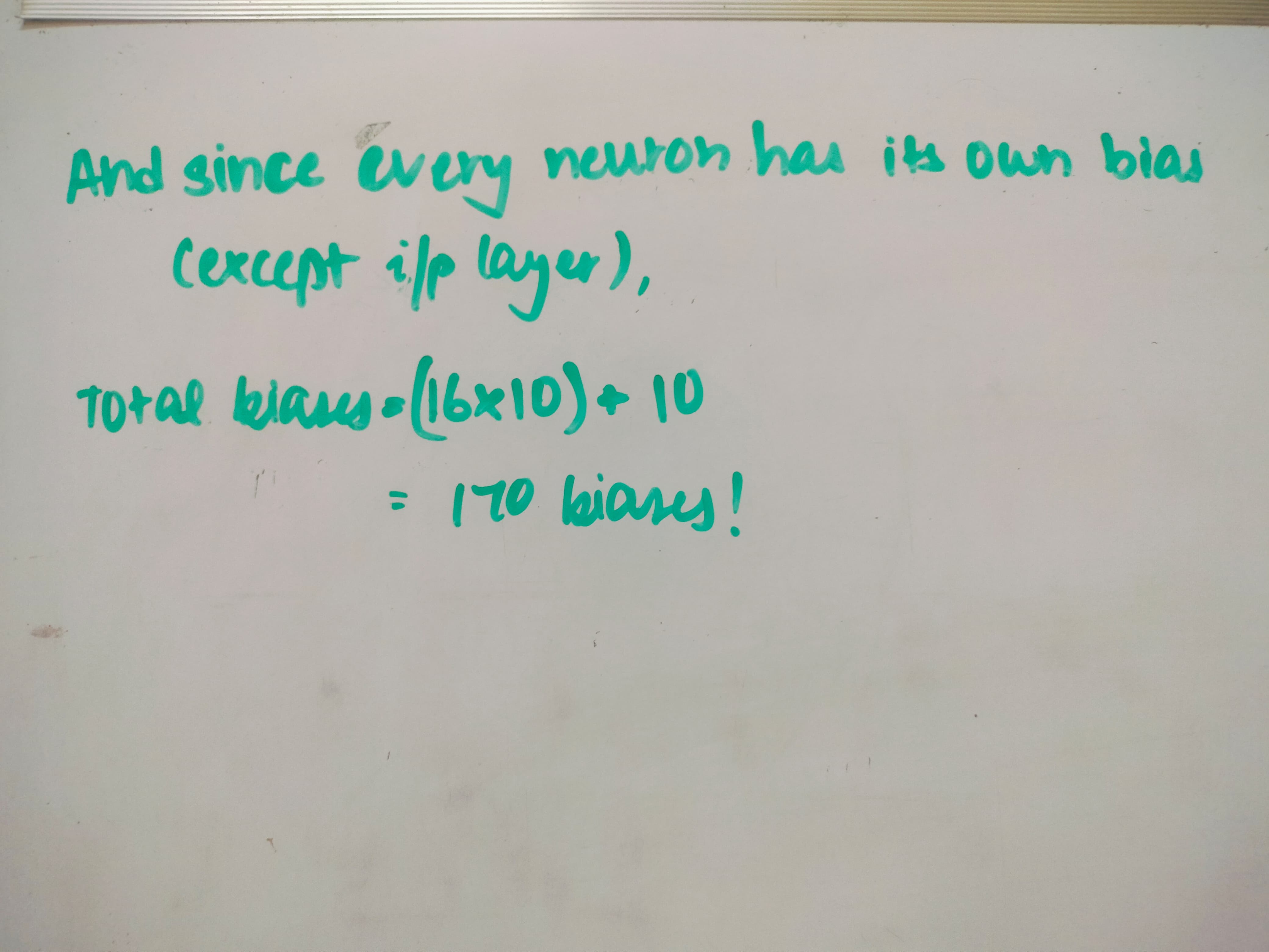
• Bias: Similar to weights, every neuron will have its own bias which will be included along with the total weighted sum. This is so that the activation can be adjusted using each individual neuron without having to adjust the entire layer of neurons, which just adds flexibility to the whole learning process.
  
  Fine, I'll calculate the thing too.
  
  
  
  
  And here's the same thing we discussed in matrix form, if that's something you're into:
  
  
  
  
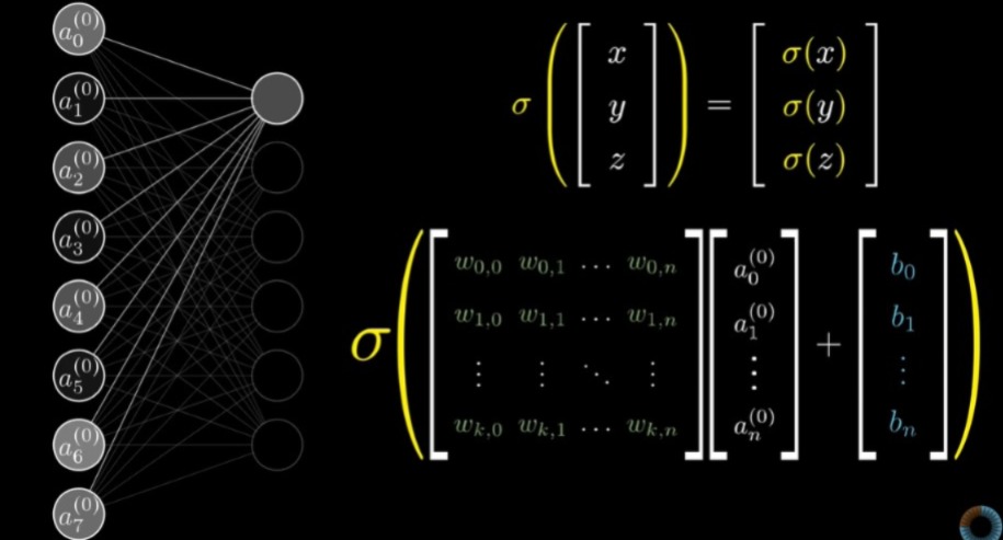
  And that wraps up the basic concept and numerical/algebraic expressions related to neural networks! We're now finally eligible to talk about the types briefly, since I think this blog is already quite yappy.
  
  

TYPES OF NEURAL NETWORKS

**1. ANN**
ANN stands for artificial neural network. It is the simplest type of neural network, and is used for simple tasks like predicting housing or simple image detection. The example we explored above is an example of an artificial neural network: Characterised by simple layers, weights and biases.
**2. CNN**
CNN stands for convolutional neural network. It is not the simplest type. That position is taken by ANNs. This one is similar, though, in the sense that it contains layers and neurons. Except these layers are convolutional and they apply filters/kernels (which are like tiny matrices/grids of numbers) over data to detect patterns. This is convolving. Next, there is a pooling process, where all this data is shrunk down. A common method is max pooling, where only the highest value in the grid is taken. This makes them suitable for image recognition applications.
**3. RNN**
RNN stands for recurrent neural network. Here, the output of each neuron is fed back to itself so that information is retained, and can be recalled when the next piece of data is input. This is useful in applications involving speech sentiment analysis, speech recognition or prediction of, say, stock prices.
**4. GAN**
GAN stands for generative adversarial network. There are two segments to this: the generator and an adversary... Just kidding, the generator and the discriminator. That was hilarious. Anyway, this type of neural network essentially works on the good-cop-bad-cop principle. The generator creates fake data that looks as real as possible, and the discriminator tries to tell the real data from the fake. This is used in applications such as image generation (changing one style to another), or creating deepfakes.
**5. Transformer Network**
While all the aforementioned neural networks take in data and process it step-by-step, transformer networks take it all at once and process the parts of the data that actually need attention, even if these parts are far apart in the given sequence. It is, hence, said to work on an attention mechanism. It is used in translation, summarisation, etc.
In conclusion, neural networks are cool and we use them a whole lot in multiple domains. And I just wrote almost 2k words about how they work on a basic level. I could go on because this topic genuinely interests me, but I decided to procrastinate writing this and now have no time left to write about all the types and applications. Thank you for coming to my TEDtype. I hope this blog post is actually comprehensible too and not just a bunch of words and pictures. Also, all credits for content, images, etc go to [this](https://www.youtube.com/watch?v=aircAruvnKk) and the ones mentioned in the resources in the MARVEL website.